Table Tennis gear shopping can be a complex endeavor. When you get to the point of getting a custom racket, combining a blade + 2 Rubbers gives you pretty high number of combinations. For example, a blade can be made of wood or wood+carbon for the most part, with a variety of combinations in terms of ply (usually 5-7) and they are classified as Defensive, Offensive and All around, with many levels in between. On the rubber side, most advanced amateur players would use different rubbers on each side, looking for different characteristics on the forehand vs backhand. Then you have the sheet’s thickness, hardness, speed, spin and style (“Chinese” vs “European”), among other characteristics.
No brand tells you “hey is rubber is meant to be used on the forehand”, because that’s up to you, given your style. This can be overwhelming when you are looking to build your first custom combo, so given my passion for table tennis + data skills + coronavirus free time, I decided to shed some light on the very pressing problem of deciding what rubber to use on which side of a racket.
For this I pulled rubber reviews from the fantastic site revspin.net, around 8500 in total. Not every review tells you whether they used/recommend the rubber for an specific side, so after some regex magic the dataset was reduced to about 3500 reviews. After this I manually labeled 500 of them with a ‘bh’, ‘fh’ or ‘both’ label to build an initial classifier, with the intention of using it to label the rest of the data and get some insights. Let’s start with the code.
reviews = pd.read_csv("bh_fh_rubber_dataset.csv")
reviews = reviews[["text","label"]]
reviews.groupby(by="label").count()/len(reviews[reviews["label"].isna()==False])
| text | |
|---|---|
| label | |
| bh | 0.521739 |
| both | 0.117202 |
| fh | 0.361059 |
reviews = reviews[(reviews["label"].isna()==False) & (reviews["label"]!="both") ]
After importing libraries and dataset, I proceed to exclude records with no label and records with the label ‘both’ since I don’t have enough labeled data yet to go the multiclass route. I’ll focus only on bh/fh labels to build a binary classifier.
#Converting to lowercase
reviews['text']=reviews['text'].apply(lambda x: x.lower())
reviews.groupby(by="label").count()/len(reviews)
| text | |
|---|---|
| label | |
| bh | 0.591006 |
| fh | 0.408994 |
I’ll consider the proportion above balanced-enough for the exercise, I’ll consider labeling more fh examples if I want to further improve the classifier.
reviews.head()
| text | label | |
|---|---|---|
| 0 | this rubber is in my opinion not as slow as in... | bh |
| 1 | i use this in 1.5mm for my backhand and it per... | bh |
| 2 | i'm using the black 1.5mm 40ª version. the ru... | bh |
| 3 | giving a fair honest review. tested this rubbe... | fh |
| 4 | i guess i got lucky with my kangaroo sheets co... | bh |
Preprocessing Link to heading
mask_fh_bh={'\\bbh\\b':'backhand',
             '\\b\back-hand\\b':'backhand',
             '\\bfh\\b':'forehand',
             '\\bfore-hand\\b':'forehand',
            'back hand': 'backhand',
            'fore hand':'forehand'
           }
reviews['text'].replace(mask_fh_bh, regex=True,inplace=True)
The above 2 cells replace shorts like bh or (bh) to “backhand” and same for forehand shorts.
# Text cleaning and text feature utility functions

def text_cleaner(string):

    string = re.sub(r'(\")', '', string)
    string = re.sub(r'(\r)', '', string)
    string = re.sub(r'(\n)', '', string)
    string = re.sub(r'(\r\n)','', string)
    string = re.sub(r'(\\)', '', string)
    string = re.sub(r'\t', '', string)
    string = re.sub(r'\:', '', string)
    string = re.sub(r'\"\"\"\"', '', string)
    string = re.sub(r'_', '', string)
    string = re.sub(r'\+', '', string)
    string = re.sub(r'\=', '', string)
    string = re.sub(r'\r\n', '', string)
    string = re.sub(r'\r\n\r\n', '', string)
    string = re.sub(r'rnrn', '', string)

    return string

def remove_accented_chars(text):
    text = unicodedata.normalize('NFKD', text).encode('ascii', 'ignore').decode('utf-8', 'ignore')
    return text

def expand_contractions(text, contraction_mapping=CONTRACTION_MAP):
    '''
    CONTRACTION_MAP is based on https://github.com/dipanjanS/practical-machine-learning-with-python/blob/master/bonus%20content/nlp%20proven%20approach/contractions.py
    '''
    contractions_pattern = re.compile('({})'.format('|'.join(contraction_mapping.keys())),
                                      flags=re.IGNORECASE|re.DOTALL)
    def expand_match(contraction):
        match = contraction.group(0)
        first_char = match[0]
        expanded_contraction = contraction_mapping.get(match)\
                                if contraction_mapping.get(match)\
                                else contraction_mapping.get(match.lower())
        expanded_contraction = first_char+expanded_contraction[1:]
        return expanded_contraction

    expanded_text = contractions_pattern.sub(expand_match, text)
    expanded_text = re.sub("'", "", expanded_text)
    return expanded_text

def remove_special_characters(text, remove_digits=True):
    pattern = r'[^a-zA-z0-9\s]' if not remove_digits else r'[^a-zA-z\s]'
    return re.sub(pattern, ' ', text)

def simple_stemmer(text):
    ps = nltk.porter.PorterStemmer()
    return ' '.join([ps.stem(word) for word in text.split()])

def simple_lemmatizer(text):
    lm = nltk.stem.WordNetLemmatizer()
    return ' '.join([lm.lemmatize(word) for word in text.split()])

# nlp = spacy.load("en_core_web_sm")
# pos_list = ['PRON','ADJ','NOUN','VERB','ADV','PROPN']

# def pos_tag_count(text):
#     c = Counter(([token.pos_ for token in nlp(text)]))
#     pos_dict = {k: v for k, v in dict(c).items() if k in pos_list}
#     return pos_dict
def text_processing(text, text_cleaner_flg=True,remove_accented_chars_flg=True,
                    expand_contractions_flg=True, remove_special_characters_flg=True,
                   simple_stemmer_flg=True, simple_lemmatizer_flg=False ):
    if text_cleaner_flg:
        text = text_cleaner(text)
    if remove_accented_chars_flg:
        text = remove_accented_chars(text)
    if expand_contractions_flg:
        text = expand_contractions(text)
    if remove_special_characters_flg:
        text = remove_special_characters(text)
    if simple_stemmer_flg:
        text = simple_stemmer(text)
    if simple_lemmatizer_flg:
        text = simple_lemmatizer(text)
    return text
I found that lemmatization and POS tagging features didn’t help with the accuracy of the classifier so I commented out those sections to keep the whole process leaner.
reviews['text']=reviews['text'].apply(text_processing)
#POS tagging features
# pos_series = reviews['text'].apply(pos_tag_count)
# pos_df = pd.DataFrame(pos_series.tolist(), index=pos_series.index)
# reviews = reviews.join(pos_df)

#filling missing values from pos tagging
#reviews.fillna(0,inplace=True)
#train_x, valid_x, train_y, valid_y = model_selection.train_test_split(reviews[['text']+pos_list], reviews['label'])
train_x, valid_x, train_y, valid_y = model_selection.train_test_split(reviews['text'], reviews['label'],test_size=0.2,random_state=0)
encoder = preprocessing.LabelEncoder()
train_y = encoder.fit_transform(train_y)
valid_y = encoder.fit_transform(valid_y)
name_mapping = dict(zip(encoder.classes_, encoder.transform(encoder.classes_)))
from sklearn.preprocessing import StandardScaler
from sklearn.compose import make_column_transformer
from sklearn.pipeline import make_pipeline
#numerical_features = train_x.dtypes == 'float'

# features = make_column_transformer(
#     (StandardScaler(), numerical_features ),
#     (make_pipeline(CountVectorizer(), TfidfTransformer()),'text')
# )

features = make_pipeline(CountVectorizer(), TfidfTransformer())
I highly recommend the use of Scikit-Learn Pipelines. The resulting code is very clean and allows for very easy experimentation/tunning with Grid Search and Cross-Validation. Now I try 4 different classifiers to explore possibilities
## Random Forest
text_clf = make_pipeline(features, RandomForestClassifier(random_state=2020))
text_clf = text_clf.fit(train_x, train_y)

predicted = text_clf.predict(valid_x)
print('Accuracy: ',np.mean(predicted == valid_y))
Accuracy: 0.8404255319148937
#SVM
text_clf_sgd = make_pipeline(features, SGDClassifier(loss='hinge', penalty='l2',
                                                alpha=1e-3, random_state=2020))

_ = text_clf_sgd.fit(train_x, train_y)
predicted_sgd = text_clf_sgd.predict(valid_x)
print('Accuracy: ',np.mean(predicted_sgd == valid_y))
Accuracy: 0.8297872340425532
#Naive Bayes
from sklearn.naive_bayes import MultinomialNB

text_clf_nb = make_pipeline(features, MultinomialNB())

_ = text_clf_nb.fit(train_x, train_y)
predicted_nb = text_clf_nb.predict(valid_x)
print('Accuracy: ',np.mean(predicted_nb == valid_y) )
Accuracy: 0.6702127659574468
#Logistic Regression
text_clf_log = make_pipeline(features, SGDClassifier(loss='log', random_state=2020))

_ = text_clf_log.fit(train_x, train_y)
predicted_log = text_clf_log.predict(valid_x)
print('Accuracy: ', np.mean(predicted_log == valid_y))
Accuracy: 0.8191489361702128
Since Random Forest and the SGD classifier are pretty close, I’ll perform hyperparameter tunning on them.
text_clf.get_params().keys()
dict_keys(['memory', 'steps', 'verbose', 'pipeline', 'randomforestclassifier', 'pipeline__memory', 'pipeline__steps', 'pipeline__verbose', 'pipeline__countvectorizer', 'pipeline__tfidftransformer', 'pipeline__countvectorizer__analyzer', 'pipeline__countvectorizer__binary', 'pipeline__countvectorizer__decode_error', 'pipeline__countvectorizer__dtype', 'pipeline__countvectorizer__encoding', 'pipeline__countvectorizer__input', 'pipeline__countvectorizer__lowercase', 'pipeline__countvectorizer__max_df', 'pipeline__countvectorizer__max_features', 'pipeline__countvectorizer__min_df', 'pipeline__countvectorizer__ngram_range', 'pipeline__countvectorizer__preprocessor', 'pipeline__countvectorizer__stop_words', 'pipeline__countvectorizer__strip_accents', 'pipeline__countvectorizer__token_pattern', 'pipeline__countvectorizer__tokenizer', 'pipeline__countvectorizer__vocabulary', 'pipeline__tfidftransformer__norm', 'pipeline__tfidftransformer__smooth_idf', 'pipeline__tfidftransformer__sublinear_tf', 'pipeline__tfidftransformer__use_idf', 'randomforestclassifier__bootstrap', 'randomforestclassifier__ccp_alpha', 'randomforestclassifier__class_weight', 'randomforestclassifier__criterion', 'randomforestclassifier__max_depth', 'randomforestclassifier__max_features', 'randomforestclassifier__max_leaf_nodes', 'randomforestclassifier__max_samples', 'randomforestclassifier__min_impurity_decrease', 'randomforestclassifier__min_impurity_split', 'randomforestclassifier__min_samples_leaf', 'randomforestclassifier__min_samples_split', 'randomforestclassifier__min_weight_fraction_leaf', 'randomforestclassifier__n_estimators', 'randomforestclassifier__n_jobs', 'randomforestclassifier__oob_score', 'randomforestclassifier__random_state', 'randomforestclassifier__verbose', 'randomforestclassifier__warm_start'])
#hide-output
from sklearn.model_selection import GridSearchCV

hyperparameters = {
                    'pipeline__countvectorizer__stop_words': ['english',None],
                    'pipeline__countvectorizer__ngram_range': [(1,1), (1,2),(2.2)],
                   'randomforestclassifier__max_depth': [50, 70],
                    'randomforestclassifier__min_samples_leaf': [1,2]
                  }
text_clf_gs = GridSearchCV(text_clf, hyperparameters, cv=5)
text_clf_gs.fit(train_x, train_y)
text_clf_gs.best_params_
{'pipeline__countvectorizer__ngram_range': (1, 1),
 'pipeline__countvectorizer__stop_words': 'english',
 'randomforestclassifier__max_depth': 70,
 'randomforestclassifier__min_samples_leaf': 1}
#refitting on entire training data using best settings

text_clf_gs.refit
preds_after_cv = text_clf_gs.best_estimator_.predict(valid_x)
np.mean(preds_after_cv == valid_y)
0.8723404255319149
RF with a jump from 84% accuracy to 87%. Now SGD.
text_clf_sgd.get_params().keys()
dict_keys(['memory', 'steps', 'verbose', 'pipeline', 'sgdclassifier', 'pipeline__memory', 'pipeline__steps', 'pipeline__verbose', 'pipeline__countvectorizer', 'pipeline__tfidftransformer', 'pipeline__countvectorizer__analyzer', 'pipeline__countvectorizer__binary', 'pipeline__countvectorizer__decode_error', 'pipeline__countvectorizer__dtype', 'pipeline__countvectorizer__encoding', 'pipeline__countvectorizer__input', 'pipeline__countvectorizer__lowercase', 'pipeline__countvectorizer__max_df', 'pipeline__countvectorizer__max_features', 'pipeline__countvectorizer__min_df', 'pipeline__countvectorizer__ngram_range', 'pipeline__countvectorizer__preprocessor', 'pipeline__countvectorizer__stop_words', 'pipeline__countvectorizer__strip_accents', 'pipeline__countvectorizer__token_pattern', 'pipeline__countvectorizer__tokenizer', 'pipeline__countvectorizer__vocabulary', 'pipeline__tfidftransformer__norm', 'pipeline__tfidftransformer__smooth_idf', 'pipeline__tfidftransformer__sublinear_tf', 'pipeline__tfidftransformer__use_idf', 'sgdclassifier__alpha', 'sgdclassifier__average', 'sgdclassifier__class_weight', 'sgdclassifier__early_stopping', 'sgdclassifier__epsilon', 'sgdclassifier__eta0', 'sgdclassifier__fit_intercept', 'sgdclassifier__l1_ratio', 'sgdclassifier__learning_rate', 'sgdclassifier__loss', 'sgdclassifier__max_iter', 'sgdclassifier__n_iter_no_change', 'sgdclassifier__n_jobs', 'sgdclassifier__penalty', 'sgdclassifier__power_t', 'sgdclassifier__random_state', 'sgdclassifier__shuffle', 'sgdclassifier__tol', 'sgdclassifier__validation_fraction', 'sgdclassifier__verbose', 'sgdclassifier__warm_start'])
#hide_output
hyperparameters_svm = { 'pipeline__countvectorizer__max_df': [0.9, 0.95],
                    'pipeline__countvectorizer__ngram_range': [(1,1), (1,2),(2.2)],
                       'pipeline__countvectorizer__stop_words': ['english',None],
                   'sgdclassifier__alpha': [0.001, 0.003,0.005],
                    'sgdclassifier__loss': ['hinge','log'],
                       'sgdclassifier__penalty':['l1','l2','elasticnet']

                  }
text_clf_sgd_cv = GridSearchCV(text_clf_sgd, hyperparameters_svm, cv=5)
text_clf_sgd_cv.fit(train_x, train_y)
text_clf_sgd_cv.best_params_
{'pipeline__countvectorizer__max_df': 0.9,
 'pipeline__countvectorizer__ngram_range': (1, 2),
 'pipeline__countvectorizer__stop_words': None,
 'sgdclassifier__alpha': 0.001,
 'sgdclassifier__loss': 'log',
 'sgdclassifier__penalty': 'l1'}
text_clf_sgd_cv.refit
preds_after_cv_sgd = text_clf_sgd_cv.best_estimator_.predict(valid_x)
np.mean(preds_after_cv_sgd == valid_y)
0.8723404255319149
Logistic regression matching Random Forest on Accuracy, now lets explore the quality of the predictions.
Model Selection Link to heading
def plot_c_matrix(models, valid_x, valid_y, label_mapping):
    for model in models:
        disp = plot_confusion_matrix(model, valid_x, valid_y,
                                 display_labels=label_mapping,
                                 cmap=plt.cm.Blues)
        title = list(model.named_steps)[1]
        disp.ax_.set_title(title)
        plt.show()
print('RF Validation Accuracy: ',np.mean(preds_after_cv == valid_y))
print('RF F1 Score: ', f1_score(valid_y, preds_after_cv))
print('SGD Validation Accuracy: ',np.mean(preds_after_cv_sgd == valid_y) )
print('SGD F1 Score:', f1_score(valid_y, preds_after_cv_sgd))
plot_c_matrix([text_clf_gs.best_estimator_,text_clf_sgd_cv.best_estimator_], valid_x, valid_y, name_mapping)
RF Validation Accuracy:  0.8723404255319149
RF F1 Score:  0.7857142857142856
SGD Validation Accuracy:  0.8723404255319149
SGD F1 Score: 0.7931034482758621
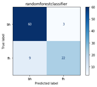
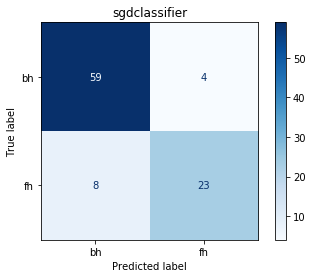
Both classifiers perform almost the same, with SGD having a better a F1 Score. Clearly the small test set is making it hard to see more clear differences.
ROC Curve Link to heading
def plot_roc(models, valid_x, valid_y):
    ns_probs = [0 for _ in range(len(valid_y))]
    ns_auc = roc_auc_score(valid_y, ns_probs)
    for model in models:
        try:
            # predict probabilities
            lr_probs = model.predict_proba(valid_x)
            # keep probabilities for the positive outcome only
            lr_probs = lr_probs[:, 1]
            lr_auc = roc_auc_score(valid_y, lr_probs)
            ns_fpr, ns_tpr, _ = roc_curve(valid_y, ns_probs)
            lr_fpr, lr_tpr, _ = roc_curve(valid_y, lr_probs)
            model_name = list(model.named_steps)[1]
            print(model_name,': ROC AUC=%.3f' % (lr_auc))
            # plot the roc curve for the model
            plt.plot(lr_fpr, lr_tpr, label=model_name)
        except AttributeError: # Error Handling for models that do not have probability prediction like svm
            continue

    plt.plot(ns_fpr, ns_tpr, linestyle='--', label='No Model')
    # axis labels
    plt.xlabel('False Positive Rate')
    plt.ylabel('True Positive Rate')
    # show the legend
    plt.legend()
    # show the plot
    plt.show()
plot_roc([text_clf_gs.best_estimator_,text_clf_sgd_cv.best_estimator_], valid_x, valid_y)
randomforestclassifier : ROC AUC=0.915
sgdclassifier : ROC AUC=0.957
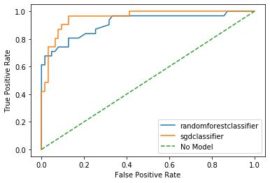
Comparing both curves SGD give us a better AUC score, which we can use to compare the quality of both classifiers. We get more predicting power with lower false alarm rate for several thresholds. We choose SGD as our to go classifier
Exploring Important Features Link to heading
feature_names_sgd = np.array(text_clf_sgd_cv.best_estimator_.named_steps.pipeline.named_steps.countvectorizer.get_feature_names())
sgd_feature_importances = np.abs(text_clf_sgd_cv.best_estimator_.named_steps.sgdclassifier.coef_[0])
sgd_idx = np.argsort(sgd_feature_importances)
y_ticks = np.arange(0, len(feature_names_sgd[sgd_idx][-15:]))
fig, ax = plt.subplots()
ax.barh(y_ticks, sgd_feature_importances[sgd_idx][-15:])
ax.set_yticklabels(feature_names_sgd[sgd_idx][-15:])
ax.set_yticks(y_ticks)
ax.set_title("SGD Feature Importances")
fig.tight_layout()
plt.show()
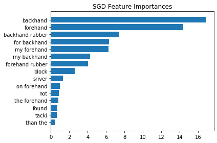
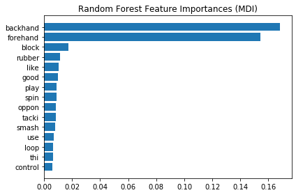
We can see here that the most important features for our classifier make total sense for our problem, with a nice surprice with “block” for example, word that is often associated with backhands on table tennis.
Exploring important features RF Link to heading
feature_names = text_clf_gs.best_estimator_.named_steps.pipeline.named_steps.countvectorizer.get_feature_names()
feature_names = np.r_[feature_names]
tree_feature_importances = text_clf_gs.best_estimator_.named_steps.randomforestclassifier.feature_importances_
sorted_idx = tree_feature_importances.argsort()
#Plotting top 10 features
y_ticks = np.arange(0, len(feature_names[-15:]))
fig, ax = plt.subplots()
ax.barh(y_ticks, tree_feature_importances[sorted_idx][-15:])
ax.set_yticklabels(feature_names[sorted_idx][-15:])
ax.set_yticks(y_ticks)
ax.set_title("Random Forest Feature Importances (MDI)")
fig.tight_layout()
plt.show()
Using model to label data Link to heading
With our classifier ready, we can use it ot label data and explore the results.
best_model = text_clf_sgd_cv.best_estimator_
def inference_review(model, text):
    '''
    Returns a prediction given an estimator and a text
    '''
    pred = model.predict([text_processing(text)])
    return encoder.inverse_transform(pred)[0]
data_4_inference = pd.read_csv('bh_fh_rubber_dataset.csv')
#Labeling all null examples, ignoring the ~500 records already labeled
data_4_inference['label'][data_4_inference['label'].isna()] = data_4_inference[data_4_inference['label'].isna()]['text'].apply(lambda text: inference_review(best_model, text))
data_4_inference = data_4_inference[data_4_inference["label"]!="both" ]
data_4_inference["rubber_name"]=data_4_inference["full_link"].str.replace("https://revspin.net/rubber/","")
data_4_inference["rubber_name"]=data_4_inference["rubber_name"].str.replace(".html","")
data_4_inference["rubber_name"]=data_4_inference["rubber_name"].str.replace("-"," ")
data_4_inference.head()
| full_link | text | label | rubber_name | |
|---|---|---|---|---|
| 0 | https://revspin.net/rubber/61-second-eagle.html | This rubber is in my opinion not as slow as in the overall rating !!!!It´s one of the softest and lightest rubber from china !!! Super controlled, very spinny and slightly tacky. Specially the ball acceptance and placement, after the service, is very easy!The sponge hardness should be realistic according to chinese scale, but I think, each rubber, around 2 degree more at the international scale (- the top rubber is medium soft).This wonderful rubber provides enough speed for my backhand (by 2 mm !!!), together with an offensive blade (by a weight of 40 g on my Timo Boll ALC) - ... this time the rubber weighs 56 g (uncut with the protective foil) and 39 g on my blade !!!Even though the sponge can be cut sometimes badly, this rubber is nevertheless very good. What I also like particularly, is that this rubber is available in three sponge hardness (36/38 & 40 degree). This allows every player to find the right partner for his blade !!!!Give me 1,8 mm too and everything would be perfect !!! - here is an additional recommendation !!! To clean the rubber I recommend isopropanol alcohol with about 66 ° percent and for the top rubber a non sticky protective film. ( ... long live, ... - rock´n roll !) ;-P | bh | 61 second eagle |
| 1 | https://revspin.net/rubber/61-second-eagle.html | I use this in 1.5mm for my backhand and it performs wonderfully. My sheet is mostly non-tacky, has a soft sponge and topsheet, with medium-large diameter pips. This combination makes flicking/looping backspin very easy. Loops, pushes, serves, and chops are all good, but blocking seems a bit inconsistent. This is likely due to my blocking skill and not the rubber though. It's a good overall rubber that I use for controlled attacking on the backhand. | bh | 61 second eagle |
| 2 | https://revspin.net/rubber/61-second-kangaroo.html | I'm using the Black 1.5mm 40ª version. The rubber is quite tacky it won't pick the ball but collects a lot of dust and give you tons of spin. Even in this thicknes is fast, i can't imagine the 2.2 version. It is difficult to glue due to it's heavy dome. it's has a lot of control on serves and chops and also suitable for BH flicks near the table but i wish the topsheet would be softer for more control so i might consider trying the 38ª version. It's a decent all arround rubber, but i wouldn't pay more than 12 dollars for it. | bh | 61 second kangaroo |
| 3 | https://revspin.net/rubber/61-second-kangaroo.html | Giving a fair honest review. Tested this rubber on a Ma Lin Extra Offensive Blade (5 ply-All Wood). Before using this rubber I was using Palio AK47-Red (FH-45 Degree Hardness) and AK47-Blue (BH-40 Degree Hardness). The Palio AK-47 sponge thickness I played with is 2.5mm. My experience with the AK-47 series is that it was a powerful rubber with almost no time for the ball to sink into the rubber. In short, it was a faster play style that is close to the table. Now with the 61 second series, I played with a 40 degree hardness on the forehand and the sponge is 2.2mm. It was slower than what I was used to, HOWEVER I gained considerable control over the ball. I bought this rubber for $8.35 USD. This is a dust magnet similar to the Hurricane 3 Neo. This rubber is not crazy fast, not too spiny, but its best quality is on control. This rubber is best for players who want to develop their strokes. .It serves well for all around playstyles. Your technique will better reflect on the result; rather than the rubber creating the result for you. This rubber is somewhat forgiving on flat hits. This rubber is good for close to the table and for players who like to hit away from the table. Overall, its a good budget rubber, Its good for beginner and intermediate (Any one under 1400 USTT rating). Anything above intermediate, there is other options that is best suited for experienced players who already know their style of play. | fh | 61 second kangaroo |
| 4 | https://revspin.net/rubber/61-second-kangaroo.html | I guess I got lucky with my kangaroo sheets compared to the other reviewers here. Mine are pretty much as advertised by 61 seconds. They're quite fast and very spinny, so if your shots are more focused on spin, they have good control. I use these for backhand rubbers and they do great. They're non-tacky with large pip diameters, which seem to make lifting backspin a bit easier. The sponge is soft with no catapult effect, so linear control can be expected. These work well for forehand also, but you really have to focus more on spin rather than speed to get the most out of them. These are still currently my preferred backhand rubber. I'm testing out the eagle as well, which seems to be as advertised also. Perhaps other reviewers are purchasing from a bad vendor? | bh | 61 second kangaroo |
pivot_t = data_4_inference.pivot_table(index=['rubber_name','label'], values='text', aggfunc='count')
total_revs = pivot_t.pivot_table(values='text', index=['rubber_name'], aggfunc=np.sum)
pivot_t = pivot_t.join(total_revs, rsuffix='_total')
pivot_t['percentage_total'] = pivot_t['text']/pivot_t['text_total']
pivot_t.sort_values(by='text_total', ascending=False ).head(16)
| text | text_total | percentage_total | ||
|---|---|---|---|---|
| rubber_name | label | |||
| dhs neo hurricane 3 | fh | 23 | 70 | 0.328571 |
| bh | 47 | 70 | 0.671429 | |
| yasaka rakza 7 | bh | 43 | 52 | 0.826923 |
| fh | 9 | 52 | 0.173077 | |
| xiom vega europe | fh | 5 | 47 | 0.106383 |
| bh | 42 | 47 | 0.893617 | |
| butterfly tenergy 05 | fh | 16 | 45 | 0.355556 |
| bh | 29 | 45 | 0.644444 | |
| donic baracuda | bh | 29 | 42 | 0.690476 |
| fh | 13 | 42 | 0.309524 | |
| yasaka rakza 7 soft | fh | 7 | 41 | 0.170732 |
| bh | 34 | 41 | 0.829268 | |
| xiom vega pro | fh | 8 | 39 | 0.205128 |
| bh | 31 | 39 | 0.794872 | |
| butterfly tenergy 64 | bh | 28 | 37 | 0.756757 |
| fh | 9 | 37 | 0.243243 |
Here we can explore the different predictions per rubber. Xiom Vega Europe is overwhelmingly used on the backhand for example, as I personally do. I do see a slight bias towards backhand predictions which make sense given that the labeled examples were 60/40 in proportion. Still not bad for ~550 examples.
Conclusion Link to heading
Very fun project to do, specially when you love the sport. We got surprising performance for such little data, my expectations before starting were way lower, I was going to be happy with 60% accuracy and ended up getting almost 90%. Eventually I realized that pre-processing was the key, like normalizing all the variations of backhand/forehand to make it easy for the classifier to pick the right feature, which we confirmed with the feature plot eventually.
Further improvement would involve more data since I labeled a very small fraction of it. Some Active Learning approach could be used to be efficient about what new examples to label. Ideally we would also aim for a more balanced dataset to avoid any source of bias. We can also combine different models and incorporate some voting system to get the predictions. Finally, this can be extended to a multiclass problem since many rubbers are used on both FH/BH, like the popular Butterfly Tenergy 05.